What are Neural Networks?
A Neural Network, vaguely inspired by the human neural networks, is a series of algorithms used by computers to determine an output based on an input of typically unfamiliar data inputs, for example pictures and sounds. A neural network is designed to ‘learn’ by itself in order to make the most accurate version of itself. The example we will use to explain the process is a number recognition neural network which determines the number in a picture, no matter how poorly drawn the number is.
Composition
It is firstly important to understand the structure of a neural network. A neural network can be visualised as many layers of ‘neurons.’ Each neurone in each layer is connected to every other neurone on its neighbouring layers.
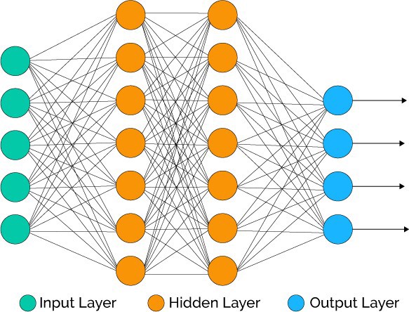
Each neurone is used to store a value from zero to one. This value signifies its ‘activation’ or how important it is to the next layer in the network (more on this later). The first layer is the input layer. In our example, each input is a pixel making up the image of the number. Each neurone holds a greyscale value for each pixel where 0 = white and 1 = black. Anywhere in between is a different shade of grey. The layers after are called the hidden layers. This is where the network applies its calculation to the input data to determine an output. Different layers tackle different aspects of the problem. In our example, one hidden layer may tackle the shape of the number whilst another tackles the edges which make up the shape. The final layer is the output layer. In our example there will be 10 different neurones in the output layer, each representing a number from 0 to 9. The neurone with the highest value will be the output as this is the number the network deems the most probable correct answer.
The Process
The inputs from the input layer are all taken into account by the first hidden layer. However an important fact is that some inputs are much more important to certain neurones in the hidden layer than others. For example, inputs coming from the corners of the image will most likely be less important than input coming from the middle of the image. Consequently, what’s known as a ‘weight’ is applied to each input going to the next neurone. A weight is a measurement of how important that input is to the neurone. At first the weights are assigned randomly, as the network has no idea what the desired values are. The value in each input neurone is multiplied by the weight and then added to the relevant neurone in the hidden layer. Another factor interpreted by the receiving neurone is a ‘bias.’ A bias is a constant added or subtracted to the end result of the inputs. It is used to control the result of the neurone – so the neurone is only significant in the next part of the network if it is necessary and reaches a certain criteria. This bias is also randomly assigned at the start. Another important thing to note is that by the time all the hundreds (or thousands) of inputs are multiplied and added to each neurone, the value will be much greater or less than the range 1 to 0. Therefore an ‘activation function’ such as ‘sigmoid derivation’ or ‘rectified linear unit’ is applied to produce a value again between zero and one. Its new activation value is now significant in the next hidden layer of the network.
Early days in the network
As we mentioned before, the initial weights and biases are randomly assigned. Consequently the first time the network is tested it should perform shockingly poorly. The value of each neurone in the hidden layer depends on three inputs: the input value from the previous neurone, the weight and the bias. We can therefore imagine each connection as a function – just massive with thousands of terms. The input values from previous neurones cannot be changed, however the weight and bias can be. Therefore it is these parameters which are adjusted to improve the performance of the neural network. The performance of the network is measured by value called a ‘cost.’ The cost is a calculation carried out on the expected results and the actual results of the network. It is the sum of the expected value minus the actual value, squared. The higher the cost, the worse the network performed. The cost can also be considered a function as it takes thousands of inputs (weights and biases) and returns a value. We want the cost to be as little as possible and since the cost is a function, we can therefore use processes similar to calculus to find what values for the parameters (weights and biases) give the minimum values for the cost.
Gradient Descent
The process of adjusting parameters to find a minimum cost is known as ‘gradient descent.’ Remembering the cost function accounts for thousands of inputs, it is difficult for the human brain to geometrically visualise, however it may look something like this:
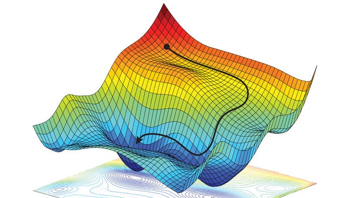
Here the cost can be lowered as parameters are changed as shown by the black line. However the problem is knowing which parameters to change in the function. To answer this, we can use the fact that some parameters are much more significant than others. For example in the equation z = 5x + y , considering the inputs will only be from 0 to 1, the coefficient of the term x is 5 times more significant than the coefficient of y and therefore adjusting this value would be more significant to the overall model. These are the parameters targeted during the learning stage of the neural network.
Back Propagation
A crucial part of the neural network development is the learning and training part. Neural networks are trained using an algorithm called ‘back propagation.’ Back propagation is used to determine how one single training example would like to adjust the values of the weights and biases of the network. A key point here is ‘would like’ – the adjustments are not based off this one example. The first step in this process is for the neural network to test and see how it does with the given sample picture. No matter how accurate the network already is, when it compares its output to the actual given value of the image it will be able find improvements in the model. As we mentioned earlier then network gives a score 0 to 1 for each of the numbers 0 to 9. After the comparison, the neural network knows that the path which results in the actual answer should give a higher score and all the other paths should give a lower score. Therefore the network will want to increase/decrease the values given by the paths before each output. It can do this 3 ways:
-
The neurones with the highest activation on the last hidden layer are the ones with most effect on the output layer – therefore the weights of these can be adjusted
-
Moreover the biases relevant to these neurones can be adjusted
-
The layer before the last hidden layer also affects the activation of the neurones on the last layer. Therefore adjusting the weights and biases leading to this layer can be adjusted to sway results.
Zooming in on the final point, going backwards deeper in the layer and changing the weights and biases will ultimately change the output at the end. This is the core principle of ‘back propagation’ and this is what the model does. It adjust all the weights and biases from the first layer to the last layer in the neural network. All of this is to reduce the overall cost of the test, therefore this is how neural networks are able to autonomously learn and perform gradient descent themselves.
Remember when we said this is how the training example ‘would like’ to adjust the values? This is important because we have to acknowledge the neural network bases these changed off on piece of example data – one number. If we allowed this then the network would only work well for that number. Therefore we run multiple tests with multiple numbers. We record how each training example ‘would like’ to change each weight and bias in the network and then find the average desired changes for each weight and biases. It is these adjustments which are actually carried out and the neural network has completed a learning generation. After the neural network has completed this process many times, it should learn, adjust and become more accurate every time. Another key point to remember is that neural networks like this are data driven – the more test data it can experiment on, the more accurate the neural network shall be. A state of the art neural network will perform at an accuracy of 99.79%.
Stochastic gradient descent
One final important part of the process is how the testing data is given to the model. If all the test data was given to the model at once and an average was found, it would most likely give the best adjustments for each weight and bias at that moment in time. However the issue with this is that it is incredibly slow. Instead, test data is randomly sorted and then split into smaller groups. The neural network then bases its averages off these smaller groups one at a time. What this means is that each adjustment is not as accurate – but will still improve the model. The advantage of this is that it happens much quicker and therefore can be repeated many times with the different groups of test data. This is called ‘Stochastic gradient descent’ and is generally a more efficient way of training the neural network.